Low voltage ride through

In electric power systems, low-voltage ride through (LVRT), or fault ride through (FRT), sometimes under-voltage ride through (UVRT), is the capability of electric generators to stay connected in short periods of lower electric network voltage (cf. voltage dip). It is needed at distribution level (wind parks, PV systems, distributed cogeneration, etc.) to avoid that a short circuit on HV or EHV level will lead to a wide-spread loss of generation. Similar requirements for critical loads such as computer systems and industrial processes are often handled through the use of an uninterruptible power supply (UPS) or capacitor bank to supply make-up power during these events.

General concept

Many generator designs use electric current flowing through windings to produce the magnetic field on which the motor or generator operates. This is in contrast to designs that use permanent magnets to generate this field instead. Such devices may have a minimum working voltage, below which the device does not work correctly, or does so at greatly reduced efficiency. Some will cut themselves out of the circuit when these conditions apply. This effect is more severe in doubly-fed induction generators (DFIG), which have two sets of powered magnetic windings, than in squirrel-cage induction generators which have only one. Synchronous generators may slip and become unstable, if the voltage of the stator winding goes down below a certain threshold.

Risk of chain reaction

In a grid containing many distributed generators subject to a low-voltage disconnection, it is possible to cause a chain reaction that takes other generators offline as well. This can occur in the event of a voltage dip that causes one of the generators to disconnect from the grid. As voltage dips are often caused by too little generation for the load in a distribution grid, removing generation can cause the voltage to drop further. This may bring the voltage down enough to cause another generator to trip, lower the voltage even further, and may cause a cascading failure.

Ride through systems

Modern large-scale wind turbines, typically 1 MW and larger, are normally required to include systems that allow them to operate through such an event, and thereby “ride through” the low voltage. Similar requirements are now becoming common on large solar power installations that likewise might cause instability in the event of a disconnect. Depending on the application the device may, during and after the dip, be required to:

disconnect temporarily from the grid, but reconnect and continue operation after the dip

stay operational and not disconnect from the grid

stay connected and support the grid with reactive power (defined as the reactive current of the positive sequence of the fundamental)

Standards

A variety of standards exist and generally vary across jurisdictions. Examples of the such grid codes are the German BDEW grid code and its supplements 2, 3, and 4 as well as the National Grid Code in UK.

Testing

Testing of the devices with less than 16 Amp rated current is described in the standard IEC 61000-4-11 and for higher current devices in IEC 61000-4-34. For wind turbines the LVRT testing is described in the standard IEC 61400-21 (2nd edition August 2008). More detailed testing procedures are stated in the German guideline FGW TR3 (Rev.22).

Anti Islanding Protection

What is Anti-Islanding?

Electric utility companies refer to residential grid-tie solar power arrays as distributed generation (DG) generators. They use this term because your solar panels are producing and distributing electrical power back into our utility grid. 

Islanding refers to the condition of a DG generator that continues to feed the circuit with power, even after power from the electric utility grid has been cut off. Islanding can pose a dangerous threat to utility workers, who may not realize that a circuit is still "live" while attempting to work on the line.

Distributed generators must detect islanding and immediately stop feeding the utility lines with power. This is known as anti-islanding. A grid-tied solar power system is required by law to have a gridtie inverter with an anti-islanding function, which senses when a power outage occurs and shuts itself off. 

One common misconception is that a grid tied system will continue to generate power during a blackout. Unless there is abattery back-up system, the gridtie solar system will not produce power when the grid is down.

The common example of islanding is a grid supply line that has solar panels attached to it. In the case of a blackout, the solar panels will continue to deliver power as long as irradiance is sufficient. In this case, the supply line becomes an "island" with power surrounded by a "sea" of unpowered lines. For this reason, solar inverters that are designed to supply power to the grid are generally required to have some sort of automatic anti-islanding circuitry in them.

In intentional islanding, the generator disconnects from the grid, and forces the distributed generator to power the local circuit. This is often used as a power backup system for buildings that normally sell their excess power to the grid.

Direct–quadrature–zero transformation

In electrical engineering, direct–quadrature–zero (or dq0 or dqo) transformation or zero–direct–quadrature (or 0dq or odq) transformation is a mathematical transformation that rotates the reference frame of three-phase systems in an effort to simplify the analysis of three-phase circuits. The dqo transform presented here is exceedingly similar to the transform first proposed in 1929 by Robert H. Park.^[1] In fact, the dqo transform is often referred to as Park’s transformation. In the case of balanced three-phase circuits, application of the dqo transform reduces the three AC quantities to two DC quantities. Simplified calculations can then be carried out on these DC quantities before performing the inverse transform to recover the actual three-phase AC results. It is often used in order to simplify the analysis of three-phase synchronous machines or to simplify calculations for the control of three-phase inverters. In analysis of three-phase synchronous machines the transformation transfers three-phase stator and rotor quantities into a single rotating reference frame to eliminate the effect of time varying inductances.

Definition

A power-invariant, right-handed dqo transform applied to any three-phase quantities (e.g. voltages, currents, flux linkages, etc.) is shown below in matrix form:^[2]

The inverse transform is:

Geometric Interpretation

The dqo transformation is two sets of axis rotations in sequence. We can begin with a 3D space where a, b, and c are orthogonal axes.

If we rotate about the a axis by -45°, we get the following rotation matrix:

,

which resolves to

.

With this rotation, the axes look like

Then we can rotate about the new b axis by about 35.26° ():

,

which resolves to

.

When these two matrices are multiplied, we get the Clarke transformation matrix C:

This is the first of the two sets of axis rotations. At this point, we can relabel the rotated a, b, and c axes as α, β, and z. This first set of rotations places the z axis an equal distance away from all three of the original a, b, and c axes. In a balanced system, the values on these three axes would always balance each other in such a way that the z axis value would be zero. This is one of the core values of the dqo transformation; it can reduce the number relevant variables in the system.

The second set of axis rotations is very simple. In electric systems, very often the a, b, and c values are oscillating in such a way that the net vector is spinning. In a balanced system, the vector is spinning about the z axis. Very often, it is helpful to rotate the reference frame such that the majority of the changes in theabc values, due to this spinning, are canceled out and any finer variations become more obvious. So, in addition to the Clarke transform, the following axis rotation is applied about the z axis:

.

Multiplying this matrix by the Clarke matrix results in the dqo transform:

.

The dqo transformation can be thought of in geometric terms as the projection of the three separate sinusoidal phase quantities onto two axes rotating with the same angular velocity as the sinusoidal phase quantities. The two axes are called the direct, or d, axis; and the quadrature or q, axis; that is, with the q-axis being at an angle of 90 degrees from the direct axis.

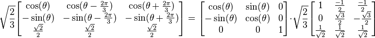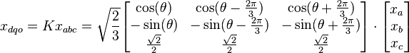
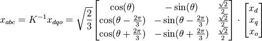
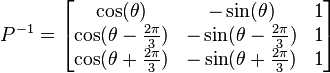
Shown above is the dqo transform as applied to the stator of a synchronous machine. There are three windings separated by 120 physical degrees. The three phase currents are equal in magnitude and are separated from one another by 120 electrical degrees. The three phase currents lag their corresponding phase voltages by . The d-q axis is shown rotating with angular velocity equal to , the same angular velocity as the phase voltages and currents. The d axis makes an angle  with the A winding which has been chosen as the reference.The currents  and  are constant DC quantities.

Comparison with other transforms

Park's transformation

The transformation originally proposed by Park differs slightly from the one given above. Park's transformation is:

and

Although useful, Park's transformation is not power invariant whereas the dqo transformation defined above is.^[2]:88 Park's transformation gives the same zero component as the method of symmetrical components. The dqo transform shown above gives a zero component which is larger than that of Park or symmetrical components by a factor of .

αβγ transform

Main article: αβγ transform

The dqo transform is conceptually similar to the αβγ transform. Whereas the dqo transform is the projection of the phase quantities onto a rotating two-axis reference frame, the αβγ transform can be thought of as the projection of the phase quantities onto a stationary two-axis reference frame.

REF:From Wikipedia, the free encyclopedia

PID controller theory

PID controller theory

This section describes the parallel or non-interacting form of the PID controller. For other forms please see the section Alternative nomenclature and PID forms.

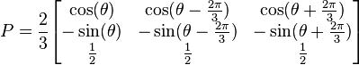
The PID control scheme is named after its three correcting terms, whose sum constitutes the manipulated variable (MV). The proportional, integral, and derivative terms are summed to calculate the output of the PID controller. Defining  as the controller output, the final form of the PID algorithm is:

where

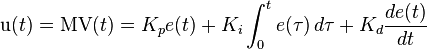
: Proportional gain, a tuning parameter

: Integral gain, a tuning parameter

: Derivative gain, a tuning parameter

: Error 

: Set Point

: Process Variable

: Time or instantaneous time (the present)

: Variable of integration; takes on values from time 0 to the present .

Equivalently, the transfer function in the Laplace Domain of the PID controller is

where

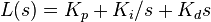
: complex number frequency

Proportional term

Plot of PV vs time, for three values of K_p (K_i and K_dheld constant)

The proportional term produces an output value that is proportional to the current error value. The proportional response can be adjusted by multiplying the error by a constant K_p, called the proportional gain constant.

The proportional term is given by:

A high proportional gain results in a large change in the output for a given change in the error. If the proportional gain is too high, the system can become unstable (see the section on loop tuning). In contrast, a small gain results in a small output response to a large input error, and a less responsive or less sensitive controller. If the proportional gain is too low, the control action may be too small when responding to system disturbances. Tuning theory and industrial practice indicate that the proportional term should contribute the bulk of the output change.^{[citation needed]}

In a real system, proportional-only control will leave an offset error in the final steady-state condition. Integral action is required to eliminate this error.

Integral term

Plot of PV vs time, for three values of K_i (K_p and K_dheld constant)

The contribution from the integral term is proportional to both the magnitude of the error and the duration of the error. The integral in a PID controller is the sum of the instantaneous error over time and gives the accumulated offset that should have been corrected previously. The accumulated error is then multiplied by the integral gain () and added to the controller output.

The integral term is given by:

The integral term accelerates the movement of the process towards setpoint and eliminates the residual steady-state error that occurs with a pure proportional controller. However, since the integral term responds to accumulated errors from the past, it can cause the present value to overshoot the setpoint value (see the section on loop tuning).

Derivative term

Plot of PV vs time, for three values of K_d (K_p and K_iheld constant)

The derivative of the process error is calculated by determining the slope of the error over time and multiplying this rate of change by the derivative gain K_d. The magnitude of the contribution of the derivative term to the overall control action is termed the derivative gain, K_d.

The derivative term is given by:

Derivative action predicts system behavior and thus improves settling time and stability of the system.^[12][13] An ideal derivative is not causal, so that implementations of PID controllers include an additional low pass filtering for the derivative term, to limit the high frequency gain and noise.^[14]Derivative action is seldom used in practice though - by one estimate in only 25% of deployed controllers^[14] - because of its variable impact on system stability in real-world applications.^[14]

Loop tuning

Tuning a control loop is the adjustment of its control parameters (proportional band/gain, integral gain/reset, derivative gain/rate) to the optimum values for the desired control response. Stability (no unbounded oscillation) is a basic requirement, but beyond that, different systems have different behavior, different applications have different requirements, and requirements may conflict with one another.

PID tuning is a difficult problem, even though there are only three parameters and in principle is simple to describe, because it must satisfy complex criteria within the limitations of PID control. There are accordingly various methods for loop tuning, and more sophisticated techniques are the subject of patents; this section describes some traditional manual methods for loop tuning.

Designing and tuning a PID controller appears to be conceptually intuitive, but can be hard in practice, if multiple (and often conflicting) objectives such as short transient and high stability are to be achieved. PID controllers often provide acceptable control using default tunings, but performance can generally be improved by careful tuning, and performance may be unacceptable with poor tuning. Usually, initial designs need to be adjusted repeatedly through computer simulations until the closed-loop system performs or compromises as desired.

Some processes have a degree of nonlinearity and so parameters that work well at full-load conditions don't work when the process is starting up from no-load; this can be corrected by gain scheduling (using different parameters in different operating regions).

Stability

If the PID controller parameters (the gains of the proportional, integral and derivative terms) are chosen incorrectly, the controlled process input can be unstable, i.e., its output diverges, with or without oscillation, and is limited only by saturation or mechanical breakage. Instability is caused by excess gain, particularly in the presence of significant lag.

Generally, stabilization of response is required and the process must not oscillate for any combination of process conditions and setpoints, though sometimesmarginal stability (bounded oscillation) is acceptable or desired.^{[citation needed]}

Mathematically, the origins of instability can be seen in the Laplace domain.^[15] The total loop transfer function is:

where

: PID transfer function

: Plant transfer function

The system is called unstable where the closed loop transfer function diverges for some .^[15] This happens for situations where . Typically, this happens when  with a 180 degree phase shift. Stability is guaranteed when  for frequencies that suffer high phase shifts. A more general formalism of this effect is known as the Nyquist stability criterion.

Optimum behavior

The optimum behavior on a process change or setpoint change varies depending on the application.

Two basic requirements are regulation (disturbance rejection – staying at a given setpoint) and command tracking (implementing setpoint changes) – these refer to how well the controlled variable tracks the desired value. Specific criteria for command tracking include rise time and settling time. Some processes must not allow an overshoot of the process variable beyond the setpoint if, for example, this would be unsafe. Other processes must minimize the energy expended in reaching a new setpoint.
REF:wikipedia